


Next: Residence time of volcanic
Up: Volcanic aerosol optical depth
Previous: Assessments of volcanic aerosol
Stratospheric transport of volcanic aerosol
Transport processes in the stratosphere seem to be very complicated and
are not known in detail.
Therefore, usually observed  patterns are used to drive GCMs
(Stenchikov et al. 1997).
Because the volcanic aerosol reaches mainly
the lower stratosphere with a maximum concentration at an
altitude about 21 km in the tropics and about 10 km in the polar regions
(Hitchmann et al., 1994), one may try to use stratospheric circulation
models to simulate aerosol distributions.
According to Plumb (1996), however, there is enough information
available to create realistic formulations of the stratospheric
transport without the necessity to solve the primitive equations.
We perform this with a non-local diffusion formalism as it is introduced
in boundary layer meteorology by
Stull (1984). Considering
patterns are used to drive GCMs
(Stenchikov et al. 1997).
Because the volcanic aerosol reaches mainly
the lower stratosphere with a maximum concentration at an
altitude about 21 km in the tropics and about 10 km in the polar regions
(Hitchmann et al., 1994), one may try to use stratospheric circulation
models to simulate aerosol distributions.
According to Plumb (1996), however, there is enough information
available to create realistic formulations of the stratospheric
transport without the necessity to solve the primitive equations.
We perform this with a non-local diffusion formalism as it is introduced
in boundary layer meteorology by
Stull (1984). Considering  equal-area latitude belts, each
containing an aerosol amount
equal-area latitude belts, each
containing an aerosol amount  (given as mass concentration)
at the time
(given as mass concentration)
at the time  , we can define a
transilient
, we can define a
transilient  matrix
  to describe the temporal evolution of a spatial pattern by
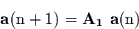 |
(4) |
where the vector  is given as
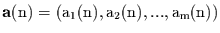 .
The initial conditions are the aerosol loading
.
The initial conditions are the aerosol loading
 in the latitude belt of eruption
  at the time of eruption
  .
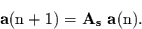
The transilient matrix does not need to be constant in time.
Instead,
the matrix rather depends on the annual cycle. Therefore we rewrite
equation (4) to introduce a dependence on the season
.
The transilient matrix does not need to be constant in time.
Instead,
the matrix rather depends on the annual cycle. Therefore we rewrite
equation (4) to introduce a dependence on the season  :
:
 |
(5) |
Note that the time step is independent from the season.
Now we consider 16 latitude belts and four seasons.
So the transilient matrix
consists of
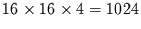 coefficients.
This seems to be a compromise between the desired spatial resolution and the
deficiency of information about the transport processes.
To decrease the
very high degree of freedom we introduce the following assumptions:
coefficients.
This seems to be a compromise between the desired spatial resolution and the
deficiency of information about the transport processes.
To decrease the
very high degree of freedom we introduce the following assumptions:
- If we assume symmetric seasons, there are only two different ones:
an extreme one (a winter- and a summer hemisphere) and a moderate one
without hemispheric differences. This reduces the amount of coefficients
in the transilient matrix to
 .
.
- If we consider very short time steps, we can apply a local
(non-isotropic) exchange. This means that only the diagonal and the first
subdiagonals of the matrix are filled with non-zero elements.
Therefore we have to
know only
 elements.
Taking also into account
the conservation of mass (i.e. the transport is without sources and sinks)
the sum over any column or row of the matrix has to be unity.
This leads to 30 independent coefficients.
elements.
Taking also into account
the conservation of mass (i.e. the transport is without sources and sinks)
the sum over any column or row of the matrix has to be unity.
This leads to 30 independent coefficients.
- According to Hitchmann et al. (1994) we can distinguish between tropics
(bordered by a pronounced mean aerosol gradient at about
 N
and S),
extratropics, and polar regions (poleward of about
N
and S),
extratropics, and polar regions (poleward of about  N and
S),
see Figure 1.
By using 16 equal-area latitude belts, there are
6 belts between
N and
S),
see Figure 1.
By using 16 equal-area latitude belts, there are
6 belts between
 representing the tropics, 8 belts that
represent the extratropics and 2 representing the polar region
(
representing the tropics, 8 belts that
represent the extratropics and 2 representing the polar region
(
 ).
).
- Now
we consider an isotropic transport within the tropics, anisotropic exchange
between tropics and extratropics, isotropic transport within the extratropics
(two seasons)
and isotropic exchange between extratropics and polar regions in the summer-
and winterhemisphere as well as during the moderate seasons.
Together with the condition of conservation of mass
this leads to only 8 independent coefficients (Table 3),
which have to be taken from or estimated from literature.
We assume that the mixing within the tropical region leads
to a nearly homogeneous distribution (less than 10% deviation from the
mean value) within 3 months after an eruption that occurs between
 latitude. This is realized by an exchange coefficient of
91% per month.
Volk et al. (1996) calculated
an entrainment rate from extratropics into tropics
of about 7% from observations. Because this value does not change between an
altitude of about 16 to 21 km we assume that this is adequate for our purpose.
The same authors found an average detrainment rate of 5% to 35%
with a pronounced altitudinal dependence. An analysis by Waugh (1996)
leads to a transport rate from the tropics to the northern hemisphere
extratropics of about 8 to 10% of the tropical mass per month. Because
the uncertainty of these estimations is about 50%, the results are in
reasonable agreement. Assuming a homogeneous aerosol distribution within
the six tropical latitude belts considered in our approximation, the exchange
coefficients from the tropical border to the extratropics follow to be
three times the transport rate per tropical mass. This leads to about
24% to 30% per month.
Considering that the distribution of aerosol within the tropics is not
exactly homogeneous we use the upper estimate as the exchange coefficient.
Boering et al. (1994) give an extratropical mixing time of about 2 to 3
months. According to this we use an extratropical exchange coefficient
of 90% per month. Then a stratospheric aerosol amount entering the extratropics
is distributed nearly homogeneously (with
latitude. This is realized by an exchange coefficient of
91% per month.
Volk et al. (1996) calculated
an entrainment rate from extratropics into tropics
of about 7% from observations. Because this value does not change between an
altitude of about 16 to 21 km we assume that this is adequate for our purpose.
The same authors found an average detrainment rate of 5% to 35%
with a pronounced altitudinal dependence. An analysis by Waugh (1996)
leads to a transport rate from the tropics to the northern hemisphere
extratropics of about 8 to 10% of the tropical mass per month. Because
the uncertainty of these estimations is about 50%, the results are in
reasonable agreement. Assuming a homogeneous aerosol distribution within
the six tropical latitude belts considered in our approximation, the exchange
coefficients from the tropical border to the extratropics follow to be
three times the transport rate per tropical mass. This leads to about
24% to 30% per month.
Considering that the distribution of aerosol within the tropics is not
exactly homogeneous we use the upper estimate as the exchange coefficient.
Boering et al. (1994) give an extratropical mixing time of about 2 to 3
months. According to this we use an extratropical exchange coefficient
of 90% per month. Then a stratospheric aerosol amount entering the extratropics
is distributed nearly homogeneously (with  deviation of the
average value) within the extratropics after 80 days.
Because circulation is more vigorous in winter and spring than in other
seasons, Hitchmann et al. (1994) found
that extratropical radiation extinction in winter-spring and summer-fall
hemispheres differ by about 20 to 50%. To consider the lower exchange in
summer and spring we assume the extratropical exchange coefficients in these
seasons to be 45% per month which is half of the winter/spring value.
The exchange coefficient between the extratropics and the summer polar region
is supposed
to be the same as the extratropical exchange coefficient in summer.
In winter the polar vortex surpresses most of the exchange. Nevertheless,
since the mean aerosol cloud in this latitude region is mainly in a height of
about 8 to 16 km (Hitchmann et al., 1994) where the polar vortex is not tight,
we assume an exchange coefficient of about 10% per month in winter time.
For spring and fall (April/May and October/November) we use an average
exchange coefficient of 23% per month.
Given the exchange coefficients between latitude belt
deviation of the
average value) within the extratropics after 80 days.
Because circulation is more vigorous in winter and spring than in other
seasons, Hitchmann et al. (1994) found
that extratropical radiation extinction in winter-spring and summer-fall
hemispheres differ by about 20 to 50%. To consider the lower exchange in
summer and spring we assume the extratropical exchange coefficients in these
seasons to be 45% per month which is half of the winter/spring value.
The exchange coefficient between the extratropics and the summer polar region
is supposed
to be the same as the extratropical exchange coefficient in summer.
In winter the polar vortex surpresses most of the exchange. Nevertheless,
since the mean aerosol cloud in this latitude region is mainly in a height of
about 8 to 16 km (Hitchmann et al., 1994) where the polar vortex is not tight,
we assume an exchange coefficient of about 10% per month in winter time.
For spring and fall (April/May and October/November) we use an average
exchange coefficient of 23% per month.
Given the exchange coefficients between latitude belt  and
and  in per cent per month
  , it is easy to get the
exchange coefficients
, it is easy to get the
exchange coefficients  in per cent per time step as
 |
(6) |
if one month equals  time steps. For practical calculations we take
180 time steps per year to fill the transilient matrix and use
time steps. For practical calculations we take
180 time steps per year to fill the transilient matrix and use
 for calculations with 60 time steps per year. Note that
is now a non-local transilient matrix.
for calculations with 60 time steps per year. Note that
is now a non-local transilient matrix.
Next: Residence time of volcanic
Up: Volcanic aerosol optical depth
Previous: Assessments of volcanic aerosol
ich
2000-01-20